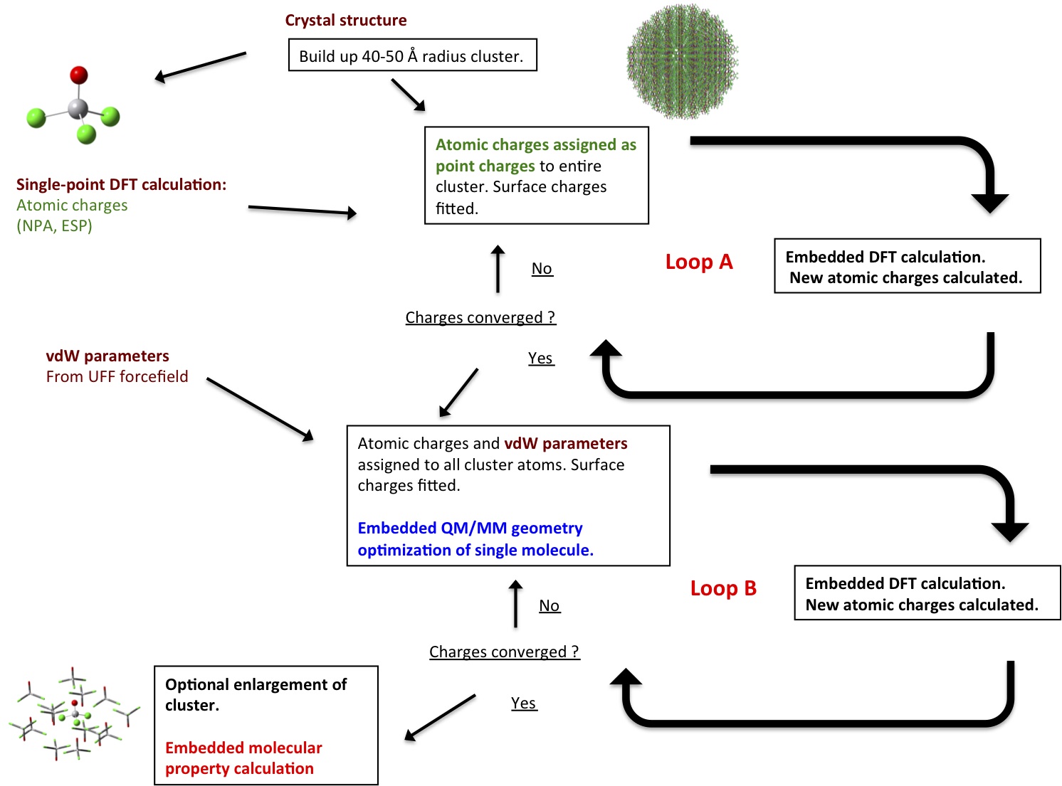
Self-consistent general QM/MM protocol for molecular crystals
The example file scfembed.chm in samples/molcrys demonstrates how to perform a self-consistent QM/MM calculation of a molecular crystal according to the protocol of Bjornsson and Bühl:
All atom charges in the protocol are stored, read and written in the Chemshell fragment files. cell.c is the unit cell fragment file, cluster.c is the working cluster fragment file (overwritten constantly) and result.c is the final optimized fragment file. Several fragment files are additionally written during the calculation: cluster-spX.c (after each single-point charge iteration) and cluster-optY-fit.c (after each geometry optimization).
1. Coordinates input
Starting from a crystal structure (here VOCl3), a spherical molecular cluster is generated (see the cutting clusters manual page). Fractional coordinates of a unit cell (without symmetrically equivalent atoms) need to be given.
Note that the connectivity of the individual molecules needs to be correct for the cluster-cutting to work (no free atoms in space). Change the chemsh_default_connectivity_toler and chemsh_default_connectivity_scale variables if necessary.
global chemsh_default_connectivity_toler
global chemsh_default_connectivity_scale
#set chemsh_default_connectivity_toler  X
#set chemsh_default_connectivity_scale  Y

c_create coords=cell.c {
cell_constants angstrom
5.02300 9.21600 11.27800 90.00000 90.00000 90.000
space_group
1
coordinates
V     0.141410    0.750000    0.954780
V     0.641410    0.750000    0.545220
V     0.858590    0.250000    0.045220
V     0.358590    0.250000    0.454780
O     0.829100    0.750000    0.950500
O     0.329100    0.750000    0.549500
O     0.170900    0.250000    0.049500
O     0.670900    0.250000    0.450500
Cl    0.255800    0.750000    0.136480
Cl    0.755800    0.750000    0.363520
Cl    0.744200    0.250000    0.863520
Cl    0.244200    0.250000    0.636480
Cl    0.273800    0.558160    0.867110
Cl    0.773800    0.941840    0.632890
Cl    0.273800    0.941840    0.867110
Cl    0.773800    0.558160    0.632890
Cl    0.726200    0.441840    0.132890
Cl    0.226200    0.058160    0.367110
Cl    0.726200    0.058160    0.132890
Cl    0.226200    0.441840    0.367110
}
2. Calculation settings
The sc-qmmm.chm file needs to be sourced to make the sc-qmmm command available. This contains all the steps of the single-point and optimization loops.
source sc-qmmm.chm
An empty file is created to create a dummy forcefield file for the single-point loop.
exec touch ./empty.ff
sc-qmmm is then called, passing in all the settings of the calculation. The script launches two bash scripts, chargeupdate-npa-orca.bash and chargecell.bash for the charge update steps. The chargeupdate-npa-orca.bash script finds the NPA charges in the output from the single-point ORCA calculation (requires gennbo, see ORCA manual).
sc-qmmm cell=cell.c   \
                     atomchargesupdate=./chargeupdate-npa-orca.bash \
                     cellchargesupdate=./chargecell.bash \
Next the size of cluster, size of active region for surface charge fitting, and atom to centre the cluster on (in cell.c) are specified:
                     radiuscluster=80 \
                     radius_active=50 \
                     originatom=1 \
The maximum number of single-point charge cycles in loop A (nsp) and optimization cycles in loop B (nopt) are specified. Loops A and B finish, however, when the RMSD of the charges between cycles change less than the value of rmscon:
                     nsp=10 \
                     nopt=10 \
                     rmscon=0.00001 \
Next, the level of theory for the single-point charge cycles in loop A is given:
                     chargelevel= [ list theory=hybrid : [ list coupling=shift  \
                                     qm_region= $qmatoms \
                                     qm_theory= orca : [ list \
                                             executable=orca \
                                               nproc=1 \
                                               hamiltonian= dft \
                                               functional=bp86 \
                                               use_ri=yes \
                                               basis=def2svp \
                                               optstr= "!NPA" \
                                               auxbasis=def2_SVP_J \
                                               gridsize=4 \
                                               finalgridsize=5 ] \
                                      mm_theory=dl_poly :  [ list  \
                                                           mxexcl= 254 \
                                                           mxlist= 20000 \
                                                           mm_defs= empty.ff  ]]] \
Finally, the level of theory for the optimization cycles in loop B:
                     optlevel= [ list tolerance=0.00045  \
                           active_atoms= $qmatoms maxcycle=700 \
                           theory=hybrid : [ list coupling=shift  \
                           qm_region= $qmatoms \
                           qm_theory= orca : [ list  \
                                               executable=orca \
                                               hamiltonian= dft \
                                               functional=bp86 \
                                               basis=def2svp \
                                               auxbasis=def2_SVP_J \
                                               use_ri=yes \
                                               gridsize=4 \
                                               finalgridsize=5 ] \
                           mm_theory=dl_poly :  [ list  \
                                             mxexcl= 254 \
                                             mxlist= 33000 \
                                             mm_defs= vocl3.ff  ]]]
The vocl3.ff file contains vdW parameters for the atoms of the system, here taken from the UFF force field.
The result.c file contains the coordinates and self-consistent charges of the full cluster with optimized coordinates of the QM region. This file (or the last input file of the QM code) can be used for a subsequent electrostatically embedded molecular property calculation.
Limitations
- The charge-update bash script is currently QM-code and charge-model specific. The current version uses ORCA and NPA charges (NPA charges performed best in our study). Can easily be modified to use other codes (Gaussian 09, Turbomole) and charge model (Mulliken, ESP charges etc.).
- Currently the scripts only work directly for homogenous crystals (i.e. all molecules in the crystal are the same). If crystal contains monoatomic counterions then the charge-updating script could easily be modified to account for this. Slighly more laborious for more complex crystals.
- The charge-update bash script used for the charge updating is currently rather inefficient.
- The vdW parameters need to be added manually to the forcefield file (as in vocl3.ff) in the optimization step. Future versions will automatically select UFF or other available vdW parameters.
Reference
- R. Bjornsson and M. Bühl, J. Chem. Theory Comput. 2012, 8, 498. DOI: 10.1021/ct200824r