Setting up the bulk MgO Cluster

Note

The scripts for this section of the tutorial can be found in li_mgo/1_construct_cluster.

1. Preparing the cluster

This section of the tutorial expands upon the ‘Modelling an MgO surface’ tutorial, in this case detailing how to set up a QM/MM cluster for bulk MgO rather than for a surface. The cluster is prepared using the script cluster_construction.py.

The periodic crystalline MgO unit cell is initially read in to ChemShell in punch format. The script cluster_construction.py reads the mgo_shells_periodic.pun punch file and creates a Fragment object containing the unit cell coordinates. As MgO is an ionic system, connect_mode is set as ionic.

# Reads in MgO crystalline unit cell in punch format
mgo=Fragment(coords="mgo_shells_periodic.pun", connect_mode='ionic')

The fragment containing the MgO unit cell is then passed to the construct_cluster() method.

# Constructs cluster
cluster=mgo.construct_cluster(origin=0, radius_cluster=20.0, 
                              adjust_charge='coordination_scaled', 
                              radius_active=12.0, bq_margin=1.5, bq_density=8)

This generates a spherical MgO cluster with a surrounding outer layer of point charges. The cutting of the cluster is determined by the origin and radius_cluster arguments:

• origin defines the atom index the cluster is centered around. Here the cluster is centered around a Mg ²⁺ ion, which is necessary for the subsequent calculations in this tutorial.

• radius_cluster defines the radius of the cluster in atomic units.

• adjust_charge adjusts the ionic charges of the outer layer ions to account for the now removed neighbouring ions. This is scaled by the coordination number (hence coordination_scaled).

Additional point charges are then fitted to reduce the error introduced by truncating the cluster. This takes the following arguments:

• radius_active sets the size for the electrostatic sampling region, and should be at least as large as the defined active MM region.

• bq_margin sets the distance between the edge of the cluster and the shell of fitted point charges.

• bq_density defines the number of point charges placed in the shell of fitted point charges.

For this model, the bq_layer parameter is not specified, as we are only concerned about the electrostatic environment of the bulk material, not the surface.

ChemShell quantifies the error introduced when truncating the cluster by its mean signed error (MSE), mean absolute error (MAE) and root-mean squared deviatation (RMSD) under the heading ‘ChemShell CLUSTER: after fitting’ in the output. These errors can be minimised by modifying the input parameters of bq_margin and bq_density. This helps ensure the distribution of the point charges surrounding the cluster is representative of the non-truncated system.

Hint

The Linux command chemsh cluster_construction.py | tee output will store the ChemShell output in a file called output as well as displaying it in the terminal. This is helpful to keep a record of changes in the error statistics!

This new cluster is then saved as a new punch file called ss-mgo_shells_cluster.pun, ready for partitioning the cluster in the next step.

Note

Alternatively the periodic input can be read from the original crystallographic information (CIF) file, using the provided cluster_construction_cif.py script.

2. Partitioning the cluster

Using the partition_cluster.py script, the cluster is partioned using the ionic embedding model. This relabels the atoms in the ss-mgo_shells_cluster.pun file with a suffix corresponding to the region they’re located in. The five regions in the ionic embedding model consist of the QM region (1), the QM/MM boundary (2), MM region (3), inactive MM (4) and the fitted point charges (5).

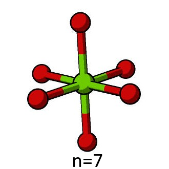
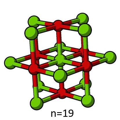
First, the QM region must be defined. This is done by defining the indices of the atoms to be included using the Python range function, specifying the first seven atoms in the pun file.

# Defines atoms to be in the QM region
n = 7
qm_region= range(0,n)

For the purposes of the tutorial, it is necessary that the electrostatics of the QM region are identical in each direction. This can only be achieved for select numbers of atoms, such as 7, 19, 27, 33 and 57. The n = 7 and n = 19 cases are the most computationally tractable options for the model, and unless specified, the n = 7 QM region will be used for all subsequent calculations in this tutorial.

Hint

For production calculations, you may wish to consider using a larger QM region for increased accuracy.

The qm_region variable is then passed as an argument in the partition() method, along with the remaining arguments which determine the partitioning of the remaining four regions.

# Partitioning the cluster
regions = mgo.partition(qm_region=qm_region, cutoff_boundary=6.0, 
                        radius_active=12.0, origin=0, 
                        qmmm_interface='explicit', interface_exclude=["O"])

• cutoff_boundary defines the width of the QM/MM interface (in atomic units), as defined as the distance from the qm_region.

• qmmm_interface specifies how the QM/MM interface is treated. ‘Explicit’ treats the atoms as BQs with attached effective core potentials (ECPs) and is the standard scheme supported by Py-ChemShell.

• interface_exclude specifies the atom symbols to be excluded from the interface. Given that the ECPs of oxygen anions are not readily available, these are excluded and are moved to the active MM region (region 3). For the purposes of the embedding model, it is sufficient to only include cations in the boundary region.

• radius_active defines the distance from the origin that atoms are assigned to the active MM region. The electrostatic sampling region used in the construction of the cluster must be at least as large as this.

After the cluster has been partioned, it is saved as a new punch file called ss-mgo_shells_regions.pun.

# Saving the new partioned cluster to disc
regions.save('ss-mgo_shells_regions.pun', 'pun')
regions.save('ss-mgo_shells_regions.xyz', 'xyz')