Calculation of the diffusion barrier
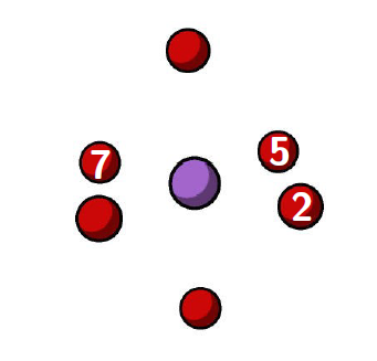
The next step in this tutorial is to calculate the diffusion barrier for the electron hole migration. To calculate the activation energy, it is necessary to calculate the minimum energy pathway for hole migration. Below, the 7 atom QM region is shown with the three of the oxygens labelled. There are two cases that can be considered for hole migration, one where the electron hole moves to an oxygen which is opposite (eg: oxygen 7-2), or alternatively where the electron hole moves to an equatorial oxygen (eg: oxygen 7-5 or oxygen 5-2). To calculate the minimum energy pathway, a nudged elastic band (NEB) calculation can be used.
It is worth highlighting that in the ‘Localising the electron hole’ section of this tutorial, the localization of the electron hole on oxygen 7 was illustrated. However, this section also requires optimized structures where the electron hole is localised on oxygens 2 and 5 as well.
1. Task-farming parallelisation
On highly distributed computer architectures, taskfarming parallelisation allows for multiple serial calculations to be performed simultaneously. This type of parallelisation is useful when large numbers of independent calculations need to be performed. This means that it is useful for NEB calculations and finite-difference Hessians, where multiple independent single point energy calculations need to be run.
For the taskfarming parallelisation, the processors are evenly divided between the specified number of workgroups. In each workgroup with \(w\) processors, there is one master process (M) and \(w-1\) worker processes (W). Each master process forms and sends tasks to the worker processes, which carry out the calculation and send the results back to the master process. To illustrate this, flowcharts are shown below for the non-taskfarmed and taskfarmed parallelisation using 16 processors and 4 workgroups.
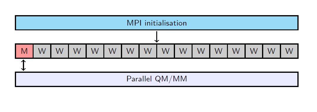
Flowchart of the non-taskfarmed parallelisation for 16 processors.
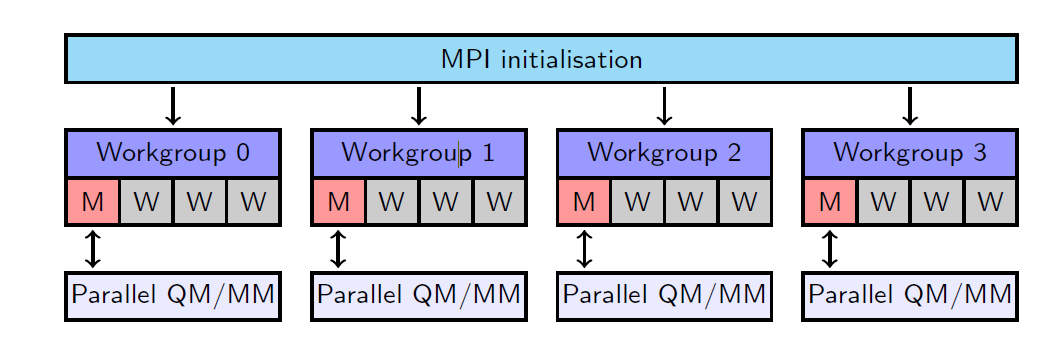
Flowchart of the taskfarmed parallelisation for 16 processors and 4 workgroups.
Task-farming parallelisation is supported by Py-ChemShell, and gives a significant advantage for calculations where computational efficiency is paramount. This type of parallelisation is useful for the subsequent calculations in this tutorial such as the nudged elastic band calculations and vibrational frequency analyses.
Note
Task-farming parallelisation requires ChemShell and NWChem to be directly linked. This will be the case on most HPC platforms, such as Hawk or ARCHER2. To run a task-farmed job, the options are specified in the Slurm submission script (see Appendix: creating a Slurm script).
2. Nudged elastic band simulations
Note
The scripts for this section of the tutorial can be found in li_mgo/3_li-mgo_neb. The O7-O2 and O7-O5
directories contain the files necessary for running the NEB calculations of the oxygen 7-2 and oxygen 7-5 hole migrations.
If you intend on running these calculations on a HPC platform, you will need to create a submission script.
The input script for the NEB is similar to that used for the geometry optimisation, as detailed in ‘Localising the electron hole’. The NEB calculation requires at least the starting and final structures to be defined, which in this case are the optimised structures where the electron holes are localised on oxygen 7 and oxygen 2 respectively.
# Imports the previously optimised localised-cluster model
rs = Fragment(coords="O7-localised.pun") # reactant structure
ps = Fragment(coords="O2-localised.pun") # product structure
The NEB is run by calling DL-FIND using the ChemShell optimisation module. Here the NEB options are specified in the Opt()
method in the script Li_MgO-cluster_NEB.py containing the arguments for the NEB.
# Runs a NEB optimisation between the defined optimised structures
opt_path = Opt(theory=qmmm, frag2=ps, neb="frozen", nimages=10,
               coordinates="cartesian", nebk=0.01, trust_radius="const",
               active=active_region)
opt_path.run()
frag2defines the end-point fragment in the reaction pathway. Here, the pre-optimised endpoint structure is specified, but if intermediate structures are known, they can be input as a python list data type to improve the initial path guess.nebkdefines the spring constant between each of the individual images.nimagesdefines the number of images along the reaction path to be requested. Two of these are the defined initial and final structures, one is the climbing image and the rest define the reaction path.neb="frozen"this option freezes the endpoints of the reaction pathway. In this case, the initial and final structures should have already been geometry optimised in order to ensure that they correspond to local minima on the energy surface.
The NEB can then be run using opt_path.run() where the reaction path is saved in the file nebpath.xyz created by DL-FIND.
The diffusion barrier can then be determined using the summary of the full reaction path located in the ChemShell output. To illustrate
this, the final output of the oxygen 7-2 hole migration is shown:
           Energy       F_tang    F_perp     Dist     Angle 1-3 Ang 1-2 Sum
Img    1   -568.9150835   0.00000   0.00000   0.14094    0.00    0.00   15.16   frozen
Img    2   -568.9146269  -0.00002   0.00008   0.14322   15.16   30.60   31.40   frozen
Img    3   -568.9134960   0.00005   0.00006   0.13778   16.24   22.09   22.43   frozen
Img    4   -568.9124546   0.00002   0.00006   0.13597    6.19    9.13    9.97   frozen
Img    5   -568.9120563  -0.00000   0.00006   0.13615    3.79    8.01   10.10   frozen
Img    6   -568.9124362  -0.00001   0.00009   0.13679    6.32   19.27   19.79   frozen
Img    7   -568.9134729  -0.00003   0.00005   0.13983   13.48   30.61   30.95   frozen
Img    8   -568.9146125  -0.00003   0.00006   0.14301   17.48    0.00   17.48   frozen
Img    9   -568.9150886   0.00000   0.00000   0.00000    0.00    0.00    0.00   frozen
Cimg   5   -568.9120721   0.00057   0.00006   0.02634    0.00    0.00    0.00
The key columns to note here are the ‘Energy’ and ‘Dist’ columns, which respectively represent the energy of the image and the distance between the given image and the next one. It is also worth highlighting that ‘Cimg’ represents the climbing image, which for the converged NEB, corresponds to the transition state.
The energy and distance parameters can thus be used to plot an energy vs reaction coordinate (R.C.) plot, where the R.C. is obtained by summing up all distances to a given image:
              Energy          R.C.
Img   1       -568.9150835    0.00000
Img   2       -568.9146269    0.14094
Img   3       -568.913496     0.28416
Img   4       -568.9124546    0.42194
Img   5       -568.9120563    0.55791
Img   6       -568.9124362    0.69406
Img   7       -568.9134729    0.83085
Img   8       -568.9146125    0.97068
Img   9       -568.9150886    1.11369
The NEB calculation can then be repeated for the oxygen 7-5 case. With the non-taskfarmed parallelisation on 4 processors, the NEB calculation should take about 60 minutes. When both of these are plotted, you should obtain a graph similar to the one shown below.
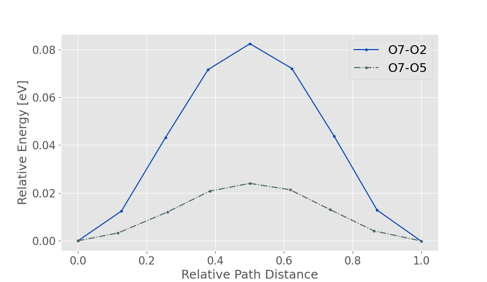
Therefore the diffusion barrier for the oxygen 7-2 parallel migration is approximately 0.082 eV (0.003 a.u) whilst the oxygen 7-5 equatorial migration is approximately 0.024 eV (0.00089 a.u). The significantly lower activation energy of the oxygen 7-5 migration illustrates how the migration between equatorial oxygens is the predominant motion in bulk Li doped MgO, and is consistent with literature findings.
Experimental literature indicates that the activation energy for this hole migration is 0.06 eV, therefore the theoretical value (0.024eV) is within chemical accuracy ( < 4 KJ/mol).