Localising the electron hole
With the MgO cluster now constructed, the structure can now be modified to produce the lithium doped cluster. When MgO is doped with lithium, the imbalance of ionic charges which manifests from substituting Mg 2+ with Li + creates an extra unoccupied hole. Literature indicates that this hole is localized to solely one oxygen, as such the active site is a [Li + O - ] center (see Wang-1986). Therefore, to create a suitable model for the subsequent calculations, it is necessary to localise the electron hole on any given oxygen.
To localise the hole, it is first necessary to generate a Li doped MgO cluster. The Li can then be displaced, and a geometry optimisation applied to find a local minima corresponding to the applied displacement. The geometry optimisation can be used in tandem with a Mulliken population analysis to determine the partial atomic charges on each oxygen and thus determine whether the electron hole is localised on one oxygen or not.
1. Localising the electron hole
Note
The scripts for this section of the tutorial can be found in li_mgo/2_li-mgo_opt/O7_localised .
To generate the Li doped MgO cluster, the first step is to read the previously constructed
ss-mgo_shells_regions.pun structure into the script Displace_Li.py.
# Defines original MgO cluster
mgo = Fragment(coords='ss-mgo_shells_regions.pun', connect_mode='ionic')
To dope the cluster with lithium, the central Mg 2+ is substitued with Li +.
The atom names and atomic numbers in the cluster can be redefined simply by changing the
names and znums labels.
# Deletes one Mg ion and substitutes with Li to form a Li-doped MgO cluster
mgo.names[0] = 'Li1'
mgo.znums[0] = 3
A small displacement of 0.4 bohr in the z axis is subsequently applied to the central Li ion. This displacement is achieved using a numpy vector which takes the cartesian coordinates of Li, and adds the corresponding numpy vector.
# Displaces the Lithium ion by a numpy vector
mgo.coords[0] += numpy.array([0, 0, 0.4])
This structure is subsequently saved in Chemshell punch format for further manipulation.
# Saves the optimized cluster to disc
mgo.save('Li_MgO-cluster.pun', 'pun')
2. Quantum Mechanics (QM)
For the subsequent calculations, NWChem requires that the basis set is specified.
The basis sets used for this tutorial are modified from the basis sets specified in the
section Single-Point Energy Calculation of the ‘Modelling an MgO surface’ tutorial.
The mgo_nwchem.basis and mgo_nwchem.ecp files were modified to include the basis set
for Li. Similar to Mg, a Stuttgart relativisitic large core basis set and ecp are used. It is worth
noting that the most diffuse functions were removed to prevent artificial spreading of charge density
into the active MM region.
The li-mgo_nwchem.basis and li-mgo_nwchem.ecp files used for all subsequent calculations in
this tutorial are shown below:
Basis sets
basis cartesian
#BASIS: Ahlrichs pVDZ
O1    S
   2266.1767785             -0.53431809926E-02
    340.87010191            -0.39890039230E-01
     77.363135167           -0.17853911985
     21.479644940           -0.46427684959
      6.6589433124          -0.44309745172
O1    S
      0.80975975668          1.0000000000
O1    S
      0.25530772234          1.0000000000
O1    P
     17.721504317            0.43394573193E-01
      3.8635505440           0.23094120765
      1.0480920883           0.51375311064
O1    P
      0.27641544411          1.0000000000
O1    D
      1.200000               1.000000
#BASIS: Modified Stuttgart RLC
Mg1 S
          2.42571930        0.02676400
          0.82262500       -0.22388000
Mg1 S
          0.10774900        0.62046400
Mg1 P
          0.76904700       -0.03664800
          0.18867500        0.24314500
Mg1 P
          0.07510100        0.55478400
#BASIS: Modified Stuttgart RLC
Li1 S
          3.0473270         0.0065550
          0.6035790        -0.1404010
Li1 S
          0.0691380         0.6237560
Li1 P
          0.8371580         0.0435070
          0.1719410         0.2296490
Li1 P
          0.0520790         0.5629490
end
Effective core potentials
ecp
 Mg1 nelec 10
 Mg1 ul
   2       1.00000000    0.00000000
 Mg1 s
   2       1.73200000   14.67600000
 Mg1 p
   2       1.11500000    5.17570000
 Mg1 d
   2       1.20300000   -1.81600000
 bq_Mg2_e nelec 0
 bq_Mg2_e ul
   2       1.00000000    0.00000000
 bq_Mg2_e s
   2       1.73200000   14.67600000
 bq_Mg2_e p
   2       1.11500000    5.17570000
 bq_Mg2_e d
   2       1.20300000   -1.81600000

 Li1 nelec 2
 Li1 ul
   2       1.000000000            0.000000000
 Li1 S
   2       1.276000000            5.786000000
 Li1 P
   2       1.607000000           -1.065000000
end
3. Geometry optimisation
The input structure used in this calculation is the Li_MgO-cluster.pun file created previously. This structure is
initially read into the script Li_MgO-cluster_optimization.py.
# Import the partioned Li_MgO cluster
li_mgo = Fragment(coords='Li_MgO-cluster.pun', connect_mode=None)
The QM region and charge of the fragment is then read in using getRegion(1) and totalcharge respectively.
The active atoms which will be relaxed for the geometry optimisation is specified using getRegion, specifying
regions 1-3 (the QM region, QM/MM interface and active MM region).
# Extracts the qm 'region' and 'charge' parameters and stores them as variables
qm_region = li_mgo.getRegion(1)
print("The QM region is ", qm_region)
qm_charge = round(li_mgo.totalcharge)
print("The QM charge is ", qm_charge)
active_region = li_mgo.getRegion(1,2,3)
print("The active region is ", active_region)
The theory for the QM/MM calculation can now be defined. The settings for the QM calculation use NWChem as the calculator,
the PBE0 hybrid functional, the charge of the QM region and the newly modified basis set and ecp files. The
argument maxiter=500 specifies for there to be up to 500 self-consistent field (SCF) cycles, instead of the default value
of 100 to help the calculation converge. A Mulliken analysis is then specified using the keyword pop_analysis='mulliken'.
qm_theory = NWChem(method='dft', functional='pbe0',
                   basis='li-mgo_nwchem.basis', ecp='li-mgo_nwchem.ecp',
                   charge=qm_charge, path='mpirun -np 4 nwchem', pop_analysis='mulliken', maxiter=500)
Caution
The path argument should be removed if you are running ChemShell and NWChem directly-linked. This is
the case for most of the high-performance computing (HPC) facilities, such as Hawk or ARCHER2. In which case,
you should specify the requested resources in the bash submission script.
The MM settings use GULP as the calculator with the mgo_2body.ff forcefield defined in the Single-Point Energy Calculation section
of ‘Modelling an MgO surface’ tutorial.
mm_theory = GULP(ff='mgo_2body.ff', conjugate=True)
The QM/MM settings are then defined. This takes the qm_theory and mm_theory options defined above as arguments. The punch file of the
structure, the coupling model (ionic) and the shell relaxation cycles are then specified. The shell maxcycles is set to a small value of 5 to
ensure timely completion of the calculation.
qmmm= QMMM(qm=qm_theory, mm=mm_theory,
           frag=li_mgo, qm_region=qm_region,
           coupling='ionic', shl_maxcycles=5)
The geometry optimisation is carried out using the standard optimisation module in PyChemShell, DL-FIND, with the settings defined in the Opt method.
# Defining the QM/MM optimization parameters
opt= Opt(theory=qmmm, algorithm="lbfgs",
         trust_radius="energy", maxcycle=200,
         maxene=300, active=active_region)

# Running QM/MM geometry optimization
opt.run()
The arguments specified in the Opt() method are defined below.
theorydetermines the theory requested for the geometry optimisation (qmmmin this case).algorithmspecifies the optimisation algorithm, which in this case is the standard lbfgs algorithm.trust_radiusspecifies the trust radius approach ('energy'bases this on the energy change).maxcycledetermines the maximum number of optimisation cycles.maxenedetermines the maximum number of energy evaluations.activespecifies the atoms in the geometry optimisation that will be relaxed. In this case, theactive_regionvariable defined earlier is specified.
The geometry optimisation is then run using opt.run() and the optimised structure is saved as Li_MgO-cluster_optimized in both punch and xyz format for further
manipulation.
# Saves the optimized Li_MgO cluster in punch and xyz formats to disc
li_mgo.save('Li_MgO-cluster_optimized.pun', 'pun')
li_mgo.save('Li_MgO-cluster_optimized.xyz', 'xyz')
4. Characterisation of the electron hole location
The Mulliken analysis results are specified in the _nwchem.out output file under the heading ‘Total Density - Mulliken Population Analysis’.
These results show the atom names, atomic numbers, charges and shell charges for each of the atoms in the QM region. The key attribute to note is the
charges on the oxygens. You should find that the charge on the oxygen with atom index 7 is significantly lower than the other oxygens. This indicates
that only oxygen 7 is electron deficient, and the electron hole is now localised.
As the partial atomic charges of the Mulliken analysis are sensitive on the choice of basis set, a more robust method of confirming the localisation
of the electron hole is to view the atomic orbital contributions to the molecular orbital which corresponds to the electron hole. If you look under the heading
‘DFT Final Beta Molecular Orbital Analysis’ in the _nwchem.out output, you will find there are a number of headings. The ‘Vector’ heading gives
the molecular orbital numbers, ‘Occ’ gives the orbital occupation and ‘E’ gives the energy of the orbital.
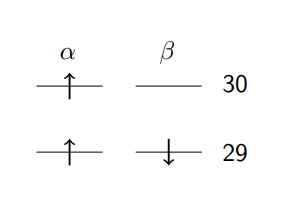
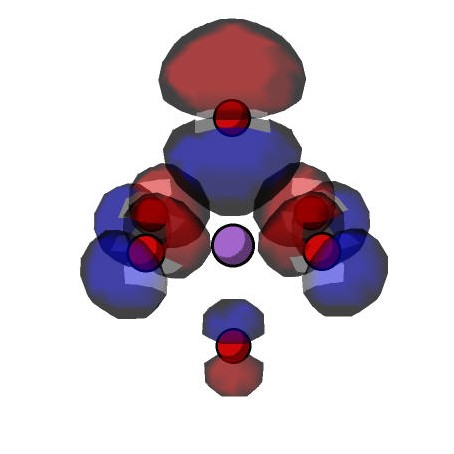
The first 30 alpha and 29 beta orbitals are occupied with one electron. Therefore, the unoccupied beta spin LUMO (orbital 30) is where the electron hole is located. You should find that the atomic orbital contribution with the highest coefficient in beta spin orbital 30 is the pz function on oxygen 7. This result is consistent with the Mulliken analysis and indicates that the hole has been successfully localised.

The beta spin 30 molecular orbital can also be plotted using DPLOT. First, the _nwchem.inp, _nwchem.db
and _nwchem.movecs input files are generated using a Py-ChemShell geometry optimisation as outlined earlier except the optimized structure is used as the input
structure. These files can be found in the DPLOT subdirectory. To the _nwchem.inp file, the following is added beneath the end keyword of the dft
section:
dplot
  TITLE o30_beta
  vectors _nwchem.movecs
   LimitXYZ
 -24.0 24.0 150
 -24.0 24.0 150
 -24.0 24.0 150
  spin beta
  orbitals view; 1; 30
  gaussian
  output o30_beta.cube
end
task dplot
The calculation can subsequently be run using NWChem. On a local machine, the command for this is nwchem _nwchem.inp. This generates a Gaussian cube file
(o30_beta.cube) which can be visualised using Jmol or other suitable open source molecular modelling packages.
The electron hole can be localised on the other oxygens simply by changing the direction of the Li displacement before carrying out the geometry optimisation. The scripts for these
are contained in the other five subdirectories in the directory li_mgo/2_li-mgo_opt.
